Briefly interpret the coefficients for G2 and absences in the context of final grade G3.
4.2 Diagnostics (minimal)
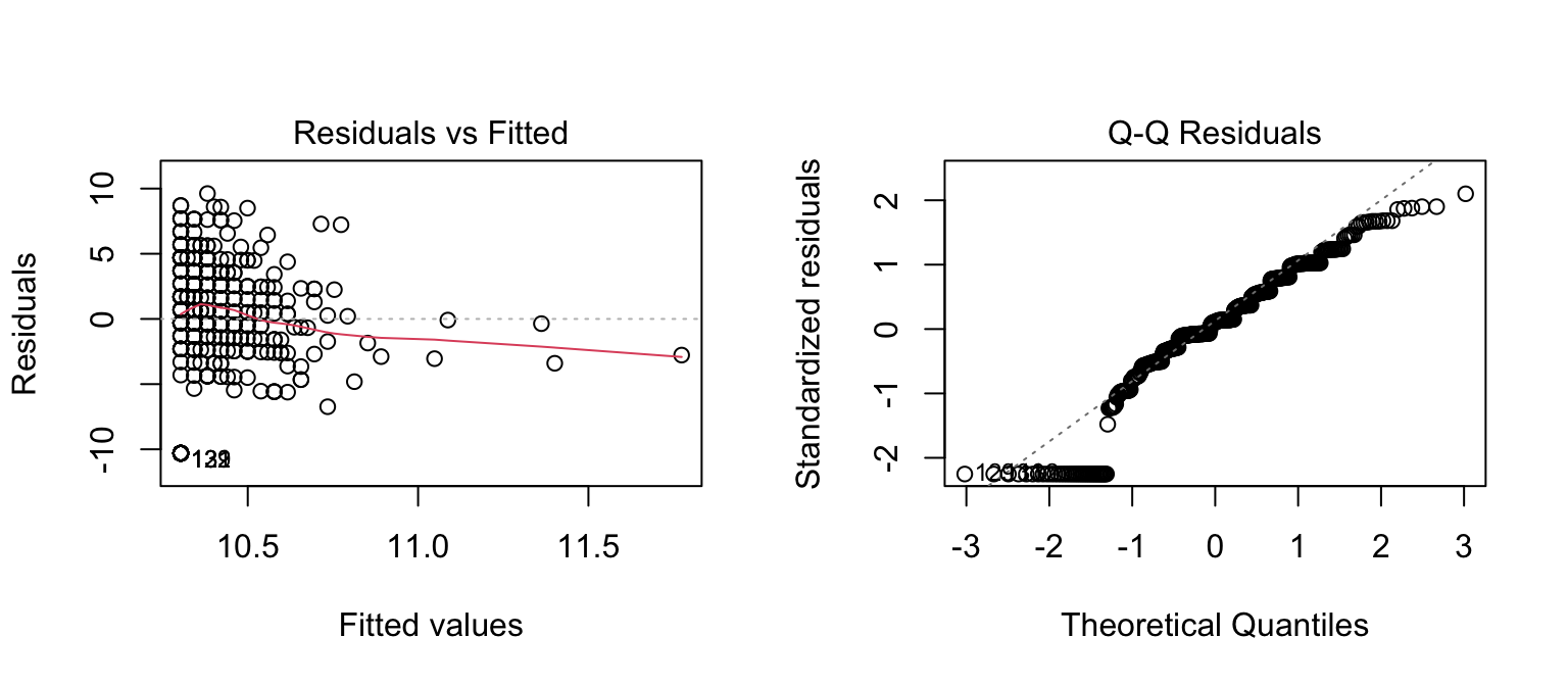
op <-par(mfrow =c(1,2))plot(basic_mod, which =1) # Residuals vs Fittedplot(basic_mod, which =2) # Normal Q-Q
par(op)
Comment on the diagnostic plots: do you see curvature, non-constant variance, or strong deviations from normality? If so, suggest a simple remedy or note the limitation.
4.3 Stepwise variable selection (student TODO)
Implement run_stepwise() in R/03_model.R using MASS::stepAIC, then try both forward and backward directions. Compare the selected model to the basic model and justify your choice.
# After you implement run_stepwise(), uncomment and run:# step_forward <- run_stepwise(analysis_data, direction = "forward")# step_backward <- run_stepwise(analysis_data, direction = "backward")# summary(step_forward)# summary(step_backward)# AIC(step_forward); AIC(step_backward)
4.4 Inference for your final model
Choose your final model (basic or one of the stepwise results) and comment on key coefficients with p-values and 95% CIs. State any caveats about interpretation.
Source Code
# Modelling and Inference {#sec-modelling}```{r}#| label: setup_03_model#| echo: false#| message: false#| warning: false#| include: falsehere::i_am("quarto/03_model.qmd")library(here)library(tidyverse)analysis_data <-readRDS(here("data", "derived", "student_performance.rda"))source(here("R", "03_model.R"))```::: {.callout-note collapse="false" icon="false" .model-instructions}<!-- BEGIN_INSTRUCTION_BLOCK -->This section guides you through classical inference for a simple linear regression. Keep your code concise and your explanations clear.Checklist1. Delete everything in this yellow callout (including BEGIN/END lines) when finished.2. Fit the provided basic model and interpret 1–2 key coefficients in plain language.3. Produce diagnostic plots and comment on linearity, constant variance, and normality.4. Implement a stepwise procedure (forward and backward) using `MASS::stepAIC` and compare to the basic model.5. Write a short paragraph interpreting coefficients, including p-values and 95% CIs, for your final chosen model.<!-- END_INSTRUCTION_BLOCK -->:::## Fit a basic regression model```{r}#| label: fit_basicbasic_mod <-fit_basic_model(analysis_data)summary(basic_mod)confint(basic_mod)```Briefly interpret the coefficients for G2 and absences in the context of final grade G3.## Diagnostics (minimal)```{r}#| label: diagnostics#| fig-width: 8#| fig-height: 3.5op <-par(mfrow =c(1,2))plot(basic_mod, which =1) # Residuals vs Fittedplot(basic_mod, which =2) # Normal Q-Qpar(op)```Comment on the diagnostic plots: do you see curvature, non-constant variance, or strong deviations from normality? If so, suggest a simple remedy or note the limitation.## Stepwise variable selection (student TODO)Implement `run_stepwise()` in `R/03_model.R` using `MASS::stepAIC`, then try both forward and backward directions. Compare the selected model to the basic model and justify your choice.```{r}#| label: stepwise# After you implement run_stepwise(), uncomment and run:# step_forward <- run_stepwise(analysis_data, direction = "forward")# step_backward <- run_stepwise(analysis_data, direction = "backward")# summary(step_forward)# summary(step_backward)# AIC(step_forward); AIC(step_backward)```## Inference for your final modelChoose your final model (basic or one of the stepwise results) and comment on key coefficients with p-values and 95% CIs. State any caveats about interpretation.