Week 4: Basic Statistical Inference

What is inference about?

Drawing conclusions about a large population on the basis of a (not necessarily large) sample
Challenge: observations based on samples are random
- We would see something different if we took a new sample
If we see a trend in the sample, how do we distinguish if it is:
- A signal: a real phenomenon that holds in the entire population
- Just noise: attributable to random chance alone

Experimental philosophy

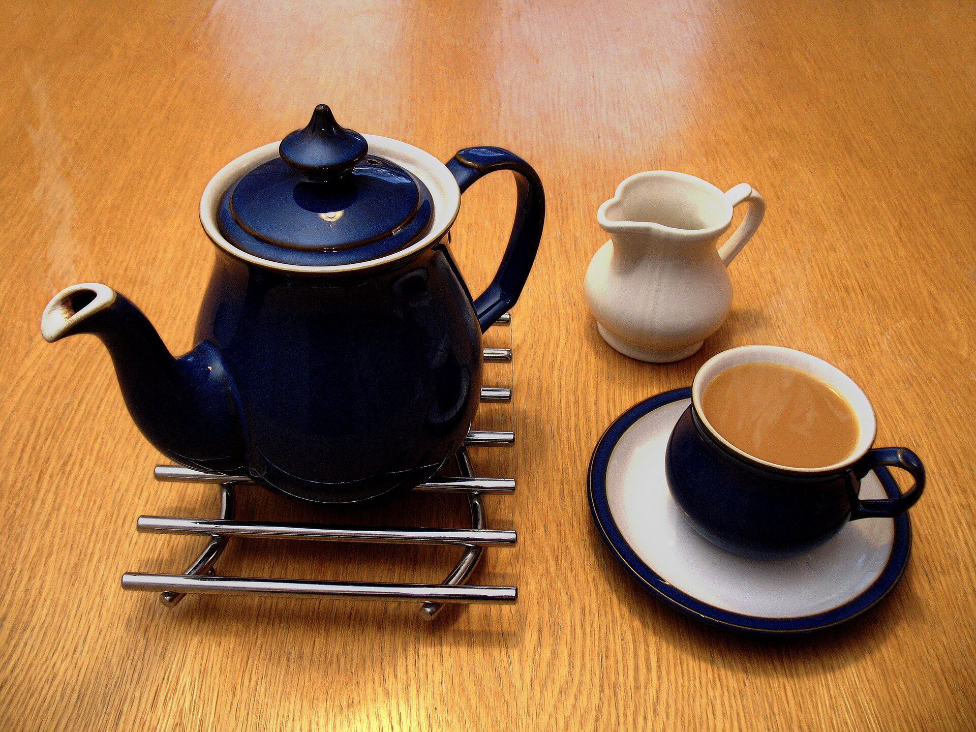
Tea tasting experiment

The claim

At a party, the topic of “milk first” versus “tea first” is being discussed
A partygoer claims she can distinguish the order in which they were poured based on taste alone

Tea tasting experiment

How to test this claim?

R.A. Fisher is widely regarded as the father of statistical inference

Another partygoer proposes to test this claim scientifically
R.A. Fisher reported on this experiment in his 1935 book The Design of Experiments

Tea tasting experiment

Formalizing the research question

In Fisher’s approach, we specify two competing hypotheses

Hypothesis	Name	Description	Interpretation
\(H_0\)	Null Hypothesis	Lady cannot distinguish tea types	Success rate = 0.5 (random guessing)
\(H_A\)	Alternative Hypothesis	Lady can distinguish tea types	Success rate > 0.5 (genuine ability)

Tea tasting experiment

Collecting data (taking a sample)

They decide on the following experiment:
- 8 cups of tea will be poured
  - 4 will have tea poured first
  - 4 will have milk poured first
These cups are presented to her in random order. Only the experimenter knows which was which.

Tea tasting experiment

Assessing the evidence

Fisher’s philosophy focuses on collecting data in order to assess the strength of evidence against \(H_0\) (i.e. in favor of \(H_A\))
i.e. how strong is the evidence that the tea taster has genuine ability

Tea tasting experiment

Assessing the evidence (to be continued…)

Once we see the data, e.g.

	True: Tea First	True: Milk First
Guess: Tea First	3	1
Guess: Milk First	1	3

Now we need to decide: are we convinced this is signal (i.e. can we rule out that it is noise)?

Statistical inference

Statistics vs. parameters

	Statistic	Parameter
Definition	A numerical summary of observed data	A characteristic of the true population-wide distribution
Symbol	Roman letters (e.g., \(\bar{x}\), \(s\), \(\hat{p}\))	Greek letters (e.g., \(\mu\), \(\sigma\), \(p\))
Known/Unknown	Known (we calculate it from our data)	Unknown (what we want to learn about)
Variability	Varies from sample to sample	Fixed (but unknown) value
Example	Sample mean height = 68.2 inches	Population mean height = \(\mu\) (unknown)

Types of parameters

Type	Symbol	Description	Example
Mean	\(\mu\)	Average value of a numeric variable in the population	Population mean height, income, test scores
Proportion	\(p\)	Fraction of population with a certain characteristic	Proportion of voters supporting a candidate
Frequency Distribution	\(\pi_1, \pi_2, \ldots\)	Proportions for each category of a categorical variable	Distribution of blood types (A, B, AB, O)

Role of models

flowchart TD
A[Unknown Population Parameters<br/>μ, σ, p, etc.] --> B[Probability Model<br/>Normal, Binomial, etc.]
B --Random sampling mechanism--> D[Observed Sample Data<br/>x₁, x₂, ..., xₙ]
D --Statistical inference--> A

style A fill:#ffcccc
style D fill:#ccffcc

Types of inference

Confidence intervals

A confidence interval provides a range of plausible values for an unknown parameter
Constructed using sample data to estimate the parameter with a specified level of confidence
Example: “We are 95% confident that the true population mean is between 2.3 and 4.7”
The confidence level (e.g., 95%) tells us how often our method would capture the true parameter if we repeated the process many times

Hypothesis tests

A hypothesis test evaluates evidence against a null hypothesis (\(H_0\))
We calculate a p-value: the probability of observing data as extreme (or more extreme) than what we saw, assuming \(H_0\) is true
Small p-values (typically < 0.05) provide strong evidence against \(H_0\)
- The significance level (e.g. \(\alpha = 0.05\)) is a pre-specified characteristic of the test: controls how convincing the evidence must be
Example: “The p-value is 0.032, so we reject \(H_0\) at the 0.05 significance level”

Duality of confidence intervals and hypothesis tests

Confidence intervals and hypothesis tests are closely related:
- If a 95% confidence interval for \(\mu\) does not contain the value \(\mu_0\), then a two-sided test of \(H_0: \mu = \mu_0\) will have p-value < 0.05
- If a 95% confidence interval does contain \(\mu_0\), then the p-value will be ≥ 0.05
Confidence intervals tell us about plausible parameter values
Hypothesis tests tell us whether specific parameter values are plausible

Cookbook for inference in R

Flowchart

flowchart TD
    A[What type of parameter?] --> B[Mean]
    A --> C[Proportion] 
    A --> D[Categorical Association]
    
    B --> E[How many groups?]
    E --> F[One sample<br/>t.test&#40;x, mu = μ₀&#41;]
    E --> G[Two samples<br/>t.test&#40;y ~ group&#41;<br/>or<br/>t.test&#40;x1, x2&#41;]
    
    C --> H[How many groups?]
    H --> I[One sample<br/>prop.test&#40;x, n, p = p₀&#41;]
    H --> J[Two samples<br/>prop.test&#40;c&#40;x1,x2&#41;, c&#40;n1,n2&#41;&#41;]
    
    D --> K[Test of independence<br/>chisq.test&#40;table&#40;var1, var2&#41;&#41;]
    
    style F fill:#e1f5fe
    style G fill:#e1f5fe
    style I fill:#f3e5f5
    style J fill:#f3e5f5
    style K fill:#e8f5e8

Examples

Single unknown mean

Example: Anorexia weight gain

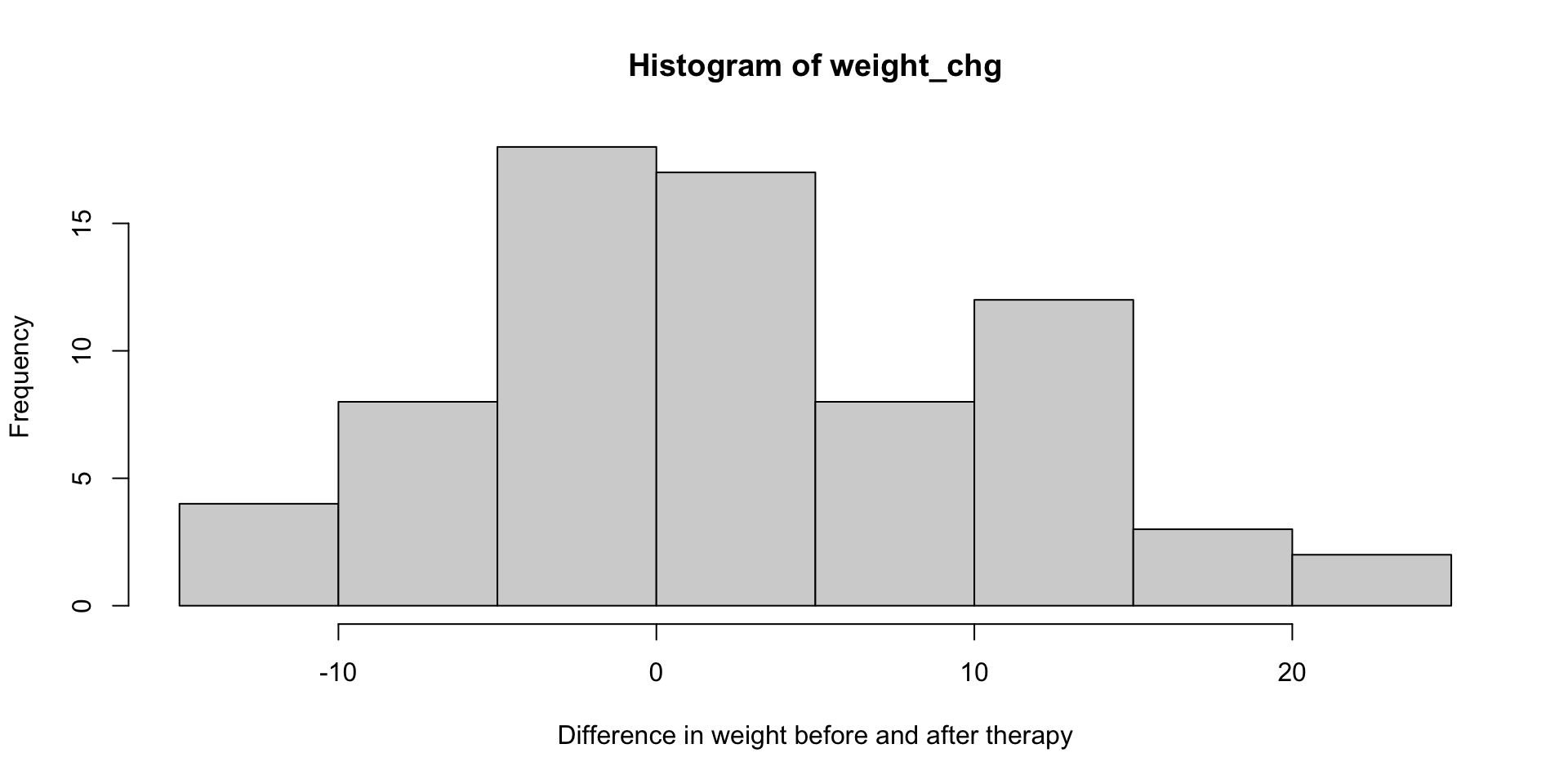
72 sampled anorexia patients receiving various therapies for their condition
For each individual, we observe their weight before and after therapy
This is a histogram of the weight changes

Load the dataset, derive the weight change, and plot

data(anorexia, package = "MASS")
weight_chg <- anorexia$Postwt - anorexia$Prewt
hist(weight_chg, xlab = "Difference in weight before and after therapy")

Parameter of interest

\(\mu\) = mean weight change among all anorexia patients
This is unknown, but:
- We do know \(\bar x\), the sample mean among these 72 patients

summary(weight_chg)

   Min. 1st Qu.  Median    Mean 3rd Qu.    Max. 
-12.200  -2.225   1.650   2.764   9.100  21.500

Among all anorexia patients, is the mean change in weight larger than zero?

Hypothesis test: formalizing the question

\(H_0: \mu = 0\), versus
\(H_A: \mu > 0\)
at level \(\alpha = 0.05\)

Hypothesis test: result

test_result <- t.test(
  x = weight_chg, # numeric vector of observations
  mu = 0, # value from H0
  alternative = "greater" # what kind of inequality is in HA
)
test_result


    One Sample t-test

data:  weight_chg
t = 2.9376, df = 71, p-value = 0.002229
alternative hypothesis: true mean is greater than 0
95 percent confidence interval:
 1.195825      Inf
sample estimates:
mean of x 
 2.763889

Outcome: The p-value is 0.002, smaller than \(\alpha = 0.05\). We reject \(H_0\).
Interpretation: There is significant evidence that the mean weight gain exceeds zero.

Confidence interval

Provide a 95% confidence interval for \(\mu\)

# do not need "mu" or "alternative" arguments here
# we do need the "level" argument
ci_result <- t.test(x = weight_chg,
                    level = 0.95) 
class(ci_result)

[1] "htest"

typeof(ci_result)

[1] "list"

names(ci_result)

 [1] "statistic"   "parameter"   "p.value"     "conf.int"    "estimate"   
 [6] "null.value"  "stderr"      "alternative" "method"      "data.name"

ci_result$conf.int

[1] 0.8878354 4.6399424
attr(,"conf.level")
[1] 0.95

Outcome: A 95% confidence interval for \(\mu\) is (0.89, 4.64)
Interpretation: We are 95% confident that the population mean weight change is between 0.89 and 4.64.

Comparing two means

Example: clinical trial

Objective: design an experiment to determine if a treatment is beneficial
Key attribute: randomization ensures that any differences between groups is attributable to treatment
- Reduces or removes confounding

flowchart LR
    A[Eligible Patients<br/>with Epilepsy] --> B[Randomization]
    B --> C[Treatment Group<br/>Progabide]
    B --> D[Control Group<br/>Placebo]
    C --> E[Measure<br/>log Seizure Rate]
    D --> F[Measure<br/>log Seizure Rate]
    E --> G[Statistical Comparison<br/>t.test&#40;log.seizure.rate ~ treatment&#41;]
    F --> G
    
    style A fill:#f9f9f9
    style B fill:#fff2cc
    style C fill:#e1f5fe
    style D fill:#ffebee
    style G fill:#f3e5f5

Outcome data from the trial

Load and display the epilepsy clinical trial data

data("epilepsy", package = "HSAUR")
epilepsy <- subset(epilepsy, period == "4")
epilepsy$log.seizure.rate <- log(1 + epilepsy$seizure.rate)
epilepsy$treatment <- relevel(epilepsy$treatment, "Progabide")
str(epilepsy)

'data.frame':   59 obs. of  7 variables:
 $ treatment       : Factor w/ 2 levels "Progabide","placebo": 2 2 2 2 2 2 2 2 2 2 ...
 $ base            : int  11 11 6 8 66 27 12 52 23 10 ...
 $ age             : int  31 30 25 36 22 29 31 42 37 28 ...
 $ seizure.rate    : int  3 3 5 4 21 7 2 12 5 0 ...
 $ period          : Ord.factor w/ 4 levels "1"<"2"<"3"<"4": 4 4 4 4 4 4 4 4 4 4 ...
 $ subject         : Factor w/ 59 levels "1","2","3","4",..: 1 2 3 4 5 6 7 8 9 10 ...
 $ log.seizure.rate: num  1.39 1.39 1.79 1.61 3.09 ...

Formalizing the research question

The question concerns the mean of the log seizure rate
- \(\mu_{\text{treatment}} = \text{mean among patients receiving the active treatment}\)
- \(\mu_{\text{placebo}} = \text{mean among patients receiving placebo}\)
We have two competing hypotheses:
- \(H_0: \mu_{\text{treatment}} = \mu_{\text{placebo}}\) (no difference)
- \(H_A: \mu_{\text{treatment}} < \mu_{\text{placebo}}\) (lower seizure rate on treatment)
We will test them at \(\alpha = 0.05\)

Assessing the evidence

test_result <- t.test(
  log.seizure.rate ~ treatment,
  data = epilepsy,
  alternative = "less"
)
test_result


    Welch Two Sample t-test

data:  log.seizure.rate by treatment
t = -1.5002, df = 56.294, p-value = 0.06958
alternative hypothesis: true difference in means between group Progabide and group placebo is less than 0
95 percent confidence interval:
       -Inf 0.04003111
sample estimates:
mean in group Progabide   mean in group placebo 
               1.541449                1.890246

Outcome: the p-value is 0.0696, which is greater than \(\alpha = 0.05\). We do not reject \(H_0\).
Interpretation: there is insufficient evidence to conclude that the mean log seizure rate among treated patients is lower than among patients receiving placebo.

Single proportion

Election poll

The October 20-23, 2024 NYT/Siena poll surveyed a random sample of 2516 likely voters nationwide.
One question asked was: if the 2024 presidential election were held today, who would you vote for?

Define and display the poll results

n <- 2516
poll_data <- tribble(
  ~candidate, ~count,
  "Kamala Harris", 1132,
  "Donald Trump", 1157,
  "All other candidates", 227
) 
poll_data$proportion <- scales::percent(poll_data$count / n, 1)

knitr::kable(poll_data)

candidate	count	proportion
Kamala Harris	1132	45%
Donald Trump	1157	46%
All other candidates	227	9%

A research question

What proportion of all likely voters at the time would vote for Kamala Harris?
Let’s construct a 95% confidence interval for this unknown proportion

Constructing a confidence interval

ci_result <- prop.test(x = 1132, n = 2516)$conf.int
ci_result

[1] 0.4303749 0.4696204
attr(,"conf.level")
[1] 0.95

We are 95% confident that between 43.0% and 47.0% of likely voters would vote for Kamala Harris

Testing a hypothesis

Among all likely voters, is the proportion of Kamala Harris voters less than 50%?
\(H_0: p = 0.5\)
\(H_A: p < 0.5\)
Test at \(\alpha = 0.05\)

Test result

prop.test(x = 1132, n = 2516, alternative = "less", p = 0.5)


    1-sample proportions test with continuity correction

data:  1132 out of 2516, null probability 0.5
X-squared = 25.04, df = 1, p-value = 2.807e-07
alternative hypothesis: true p is less than 0.5
95 percent confidence interval:
 0.0000000 0.4664785
sample estimates:
        p 
0.4499205

The p-value is extremely small (less than \(\alpha = 0.05\))
There is convincing evidence that less than 50% of likely voters favor Kamala Harris

Comparing two proportions

Arthritis trial example

flowchart LR
    A[Eligible Patients<br/>with arthritis] --> B[Randomization]
    B --> C[Treatment]
    B --> D[Placebo]
    C --> E[Proportion of patients<br/>showing marked symptom improvement]
    D --> F[Proportion of patients<br/>showing marked symptom improvement]
    E --> G[Statistical Comparison<br/>prop.test]
    F --> G
    
    style A fill:#f9f9f9
    style B fill:#fff2cc
    style C fill:#e1f5fe
    style D fill:#ffebee
    style G fill:#f3e5f5

Trial outcome data

Load the patient-level data

if(!"vcd" %in% installed.packages()) install.packages("vcd")
data("Arthritis", package = "vcd")
str(Arthritis)

'data.frame':   84 obs. of  5 variables:
 $ ID       : int  57 46 77 17 36 23 75 39 33 55 ...
 $ Treatment: Factor w/ 2 levels "Placebo","Treated": 2 2 2 2 2 2 2 2 2 2 ...
 $ Sex      : Factor w/ 2 levels "Female","Male": 2 2 2 2 2 2 2 2 2 2 ...
 $ Age      : int  27 29 30 32 46 58 59 59 63 63 ...
 $ Improved : Ord.factor w/ 3 levels "None"<"Some"<..: 2 1 1 3 3 3 1 3 1 1 ...

Formalizing the research question

Is the probability of marked symptom improvement higher on treatment than placebo?
\(H_0: p_{\text{treatment}} = p_{\text{placebo}}\)
\(H_A: p_{\text{treatment}} > p_{\text{placebo}}\)
Test at \(\alpha = 0.05\)

Trial outcome data

counts <- with(
  Arthritis,
  table(Treatment, Improved == "Marked",
        dnn = list("treatment", "marked_improvement"))
)
counts

         marked_improvement
treatment FALSE TRUE
  Placebo    36    7
  Treated    20   21

prop.table(counts, margin = 1)

         marked_improvement
treatment     FALSE      TRUE
  Placebo 0.8372093 0.1627907
  Treated 0.4878049 0.5121951

class(counts)

[1] "table"

Testing the hypotheses

Here we pass the table object as the first argument to prop.test()

prop.test(
  counts[c("Treated", "Placebo"),
         c("TRUE", "FALSE")],
  alternative = "greater"
)


    2-sample test for equality of proportions with continuity correction

data:  counts[c("Treated", "Placebo"), c("TRUE", "FALSE")]
X-squared = 10.012, df = 1, p-value = 0.0007778
alternative hypothesis: greater
95 percent confidence interval:
 0.1672693 1.0000000
sample estimates:
   prop 1    prop 2 
0.5121951 0.1627907

The p-value is small (less than \(\alpha = 0.05\)). We reject \(H_0\). There is strong evidence that the response rate is higher among treated patients than patients receiving placebo.

Producing a confidence interval

For the difference in two proportions

ci_result <- prop.test(counts)$conf.int
ci_result

[1] 0.1369409 0.5618679
attr(,"conf.level")
[1] 0.95

We are 95% confident that the difference in response rates (treatment versus placebo) is between 13.7% and 56.2%.

Associations with categorical data

Titanic example

Load and display the Titanic survival data

data("Titanic", package = "datasets")
str(Titanic)

 'table' num [1:4, 1:2, 1:2, 1:2] 0 0 35 0 0 0 17 0 118 154 ...
 - attr(*, "dimnames")=List of 4
  ..$ Class   : chr [1:4] "1st" "2nd" "3rd" "Crew"
  ..$ Sex     : chr [1:2] "Male" "Female"
  ..$ Age     : chr [1:2] "Child" "Adult"
  ..$ Survived: chr [1:2] "No" "Yes"

The research question

Does the probability of surviving the wreck depend on class?
Preparing the data (marginalizing over other factors)

class_table <- margin.table(Titanic, c("Class", "Survived"))
class_table

      Survived
Class   No Yes
  1st  122 203
  2nd  167 118
  3rd  528 178
  Crew 673 212

Formalizing

Is the distribution of survival independent of class?
\(H_0: \text{survival is independent of class}\)
\(H_A: \text{survival is NOT independent of class}\)
Test at \(\alpha = 0.05\)

Carrying out the test

chisq.test(class_table)


    Pearson's Chi-squared test

data:  class_table
X-squared = 190.4, df = 3, p-value < 2.2e-16

The p-value is very small. We reject \(H_0\). There is strong evidence that the survival is not independent from class

Returning to the tea-tasting example

Tea tasting experiment

The hypotheses

Hypothesis	Name	Description	Interpretation
\(H_0\)	Null Hypothesis	Lady cannot distinguish tea types	Success rate = 0.5 (random guessing)
\(H_A\)	Alternative Hypothesis	Lady can distinguish tea types	Success rate > 0.5 (genuine ability)

The experimental data

	True: Tea First	True: Milk First
Guess: Tea First	3	1
Guess: Milk First	1	3

Preparing the data

outcome <- matrix(
  c(3, 1,
    1, 3),
  nrow = 2, ncol = 2,
  byrow = TRUE, dimnames = list(guess = c("tea first", "milk first"),
                                truth = c("tea first", "milk first"))
)
outcome

            truth
guess        tea first milk first
  tea first          3          1
  milk first         1          3

Assessing the strength of evidence

Fisher used Fisher’s exact test (which we will not cover in the class - still you should be able to interpret the resulting p-value)

fisher.test(outcome, alternative = "greater")


    Fisher's Exact Test for Count Data

data:  outcome
p-value = 0.2429
alternative hypothesis: true odds ratio is greater than 1
95 percent confidence interval:
 0.3135693       Inf
sample estimates:
odds ratio 
  6.408309

The p-value is large (larger than \(\alpha = 0.05\)). We do not reject \(H_0\). There is insufficient evidence to conclude the lady can distinguish tea types better than random guessing.