Week 3: Descriptive Statistics and Summarizing Data

Refresher I

Class and type

We can use class() and typeof(), respectively, to determine the class and basic type of an object

data(diamonds, package = "ggplot2") # load an example dataset
class(diamonds) # inherits from data.frame, among other classes

[1] "tbl_df"     "tbl"        "data.frame"

typeof(diamonds) # basic type is a list

[1] "list"

Refresher II

Basic structure

The str() function produces a concise summary of the structure of the object

str(diamonds)

Classes 'tbl_df', 'tbl' and 'data.frame':   53940 obs. of  10 variables:
 $ carat  : num  0.23 0.21 0.23 0.29 0.31 0.24 0.24 0.26 0.22 0.23 ...
 $ cut    : Ord.factor w/ 5 levels "Fair"<"Good"<..: 5 4 2 4 2 3 3 3 1 3 ...
 $ color  : Ord.factor w/ 7 levels "D"<"E"<"F"<"G"<..: 2 2 2 6 7 7 6 5 2 5 ...
 $ clarity: Ord.factor w/ 8 levels "I1"<"SI2"<"SI1"<..: 2 3 5 4 2 6 7 3 4 5 ...
 $ depth  : num  61.5 59.8 56.9 62.4 63.3 62.8 62.3 61.9 65.1 59.4 ...
 $ table  : num  55 61 65 58 58 57 57 55 61 61 ...
 $ price  : int  326 326 327 334 335 336 336 337 337 338 ...
 $ x      : num  3.95 3.89 4.05 4.2 4.34 3.94 3.95 4.07 3.87 4 ...
 $ y      : num  3.98 3.84 4.07 4.23 4.35 3.96 3.98 4.11 3.78 4.05 ...
 $ z      : num  2.43 2.31 2.31 2.63 2.75 2.48 2.47 2.53 2.49 2.39 ...

Refresher III

Subsetting a column from a data frame

We can use $ or [[ to subset columns from a data frame

str(diamonds$price) # structure of the "price" variable

 int [1:53940] 326 326 327 334 335 336 336 337 337 338 ...

identical(diamonds$price, diamonds[["price"]])

[1] TRUE

We could define a new variable to take the value of the column

price <- diamonds$price
identical(price, diamonds$price)

[1] TRUE

Refresher IV

Type coercion

If we wanted, we could coerce this integer object to a different type

price_num <- as.numeric(price)
str(price_num)

 num [1:53940] 326 326 327 334 335 336 336 337 337 338 ...

price_chr <- as.character(price)
str(price_chr)

 chr [1:53940] "326" "326" "327" "334" "335" "336" "336" "337" "337" "338" ...

Refresher V

Aside about memory efficiency

Coercion to numeric or character would not be very advantageous in this case, and would come with a downside: the integer version takes up far less memory

object.size(price)

215808 bytes

object.size(price_num)

431568 bytes

object.size(price_chr)

1081280 bytes

What does the dataset look like?

Printout of the diamonds data

library(DT) # for the tabular display
DT::datatable(diamonds, options = list(pageLength = 5))

What are some questions we might pose about these data?

Interlude: statistical terminology refresher

What is a population?

A large group of individuals or units{.incremental}
- May be difficult to measure everyone{.incremental}
- Still would like to draw conclusions about the large group, perhaps based on partial data{.incremental}

What is a distribution?

The distribution of a measurement refers to the relative frequencies or *prevalence of different possible values across individuals in the population{.incremental}

What is a sample?

A set of measured individuals or units{.incremental}
“Sample” may also refer to the measurements themselves{.incremental}

What is a statistic?

Any function of the sample{.incremental}
For example, a numerical summary of the sample{.incremental}

Descriptive statistics

What are Descriptive Statistics?

Statistics¹ describing the main features of a dataset
Help us understand the distribution, center, and spread of data.

Types of Descriptive Statistics

Measures of Center: Mean, Median, Mode
Measures of Spread: Range, Variance, Standard Deviation, IQR
Shape: Skewness, Kurtosis
Frequency Tables: Counts and proportions for categorical variables

Summarizing Numeric Data

Measures of Center

Mean: Arithmetic average
Median: Middle value
Mode: Most frequent value

x <- c(1, 2, 2, 3, 4)
mean(x)

[1] 2.4

median(x)

[1] 2

# Mode is not built-in; use table(x)

Measures of Spread

Range: Difference between max and min
Variance: Average squared deviation from mean
Standard Deviation: Square root of variance
IQR: Interquartile range (Q3 - Q1)

range(x)

[1] 1 4

var(x)

[1] 1.3

sd(x)

[1] 1.140175

IQR(x)

[1] 1

Summarizing Categorical Data

Frequency Tables

Use table() to count occurrences
Use prop.table() for proportions

species <- c("Adelie", "Chinstrap", "Adelie", "Gentoo")
table(species)

species
   Adelie Chinstrap    Gentoo 
        2         1         1

prop.table(table(species))

species
   Adelie Chinstrap    Gentoo 
     0.50      0.25      0.25

Back to the Diamonds Dataset

Recalling the structure

str(diamonds)

Classes 'tbl_df', 'tbl' and 'data.frame':   53940 obs. of  10 variables:
 $ carat  : num  0.23 0.21 0.23 0.29 0.31 0.24 0.24 0.26 0.22 0.23 ...
 $ cut    : Ord.factor w/ 5 levels "Fair"<"Good"<..: 5 4 2 4 2 3 3 3 1 3 ...
 $ color  : Ord.factor w/ 7 levels "D"<"E"<"F"<"G"<..: 2 2 2 6 7 7 6 5 2 5 ...
 $ clarity: Ord.factor w/ 8 levels "I1"<"SI2"<"SI1"<..: 2 3 5 4 2 6 7 3 4 5 ...
 $ depth  : num  61.5 59.8 56.9 62.4 63.3 62.8 62.3 61.9 65.1 59.4 ...
 $ table  : num  55 61 65 58 58 57 57 55 61 61 ...
 $ price  : int  326 326 327 334 335 336 336 337 337 338 ...
 $ x      : num  3.95 3.89 4.05 4.2 4.34 3.94 3.95 4.07 3.87 4 ...
 $ y      : num  3.98 3.84 4.07 4.23 4.35 3.96 3.98 4.11 3.78 4.05 ...
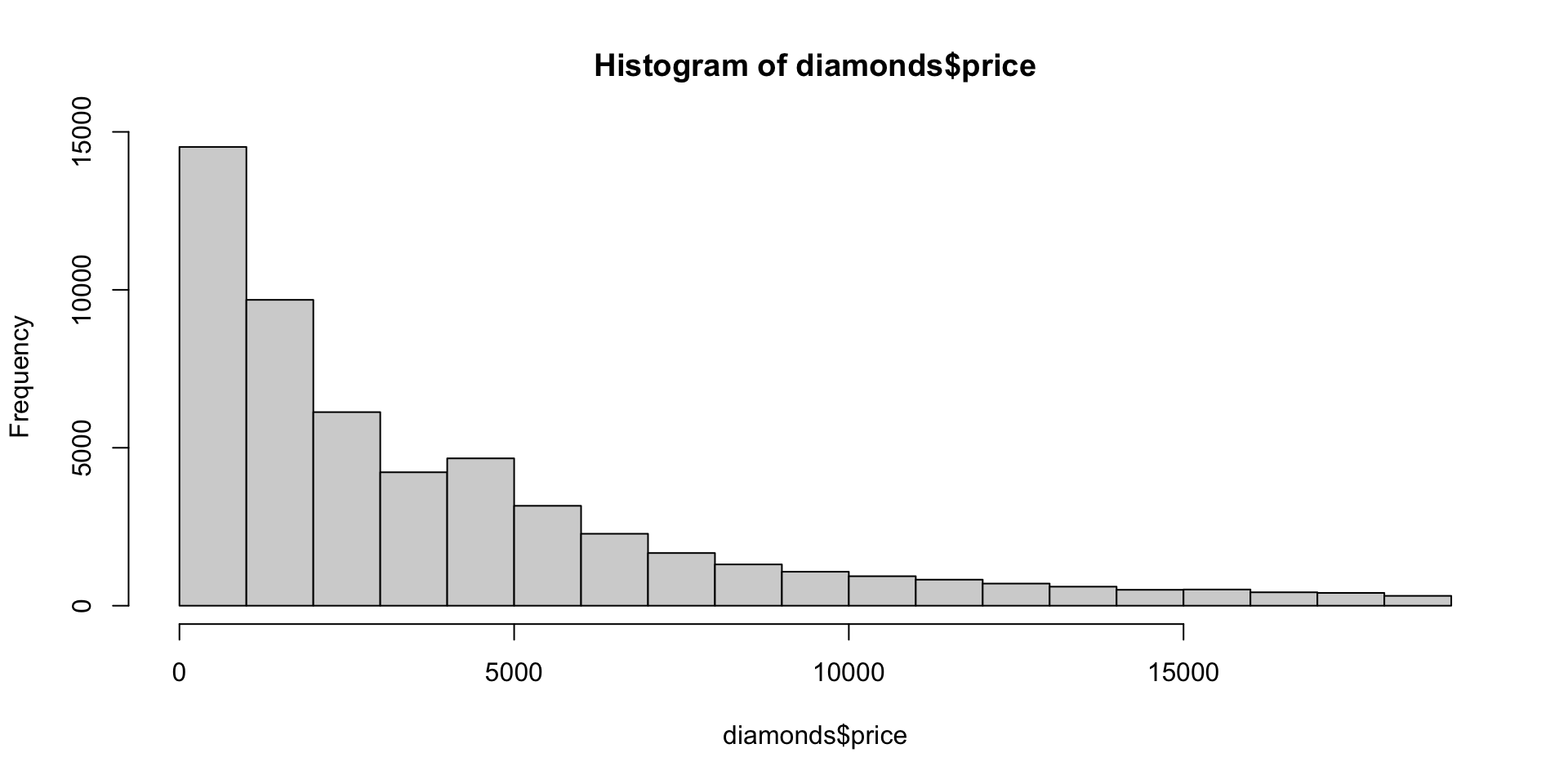
 $ z      : num  2.43 2.31 2.31 2.63 2.75 2.48 2.47 2.53 2.49 2.39 ...

Diamond price

Measures of center

What is the average price (sample mean price)?

mean(diamonds$price)

[1] 3932.8

What is a representative price? (Median)

median(diamonds$price)

[1] 2401

Diamond price

Measures of spread

Range of values

range(diamonds$price)

[1]   326 18823

Standard deviation and variance

sd(diamonds$price)

[1] 3989.44

var(diamonds$price)

[1] 15915629

sd(diamonds$price) == sqrt(var(diamonds$price))

[1] TRUE

Diamond price

Measures of spread

Quartiles: the summary() function returns the quartiles, among other information

summary(diamonds$price)

   Min. 1st Qu.  Median    Mean 3rd Qu.    Max. 
    326     950    2401    3933    5324   18823

Interquartile range

IQR(diamonds$price)

[1] 4374.25

Diamond price

Shape

A histogram is a visual display of the distribution of a scale variable

hist(diamonds$price)

Diamond price

Shape

Based on the histogram and the earlier descriptive statistics, describe the shape of the distribution of diamond prices
- Unimodal
- Right skewed
- Mean price is 3932.8 USD
- Standard deviation is 3989.44 USD
- Middle 50% of diamonds range in price from 950 USD to 5324 USD (see summary(diamonds$price))

Diamond cut quality

The `cut` variable

This is an example of a categorical variable

str(diamonds$cut) # its class in R is a factor

 Ord.factor w/ 5 levels "Fair"<"Good"<..: 5 4 2 4 2 3 3 3 1 3 ...

The possible levels of the cut variable are:

levels(diamonds$cut)

[1] "Fair"      "Good"      "Very Good" "Premium"   "Ideal"

Diamond cut quality

Frequency table

The frequency table below tells us how common each cut quality is within the sample

table(diamonds$cut)


     Fair      Good Very Good   Premium     Ideal 
     1610      4906     12082     13791     21551

Q: What is the most common cut (the mode)? Which cut appears least often in the dataset?

Diamond cut quality

Proportion table (relative frequency)

Rather than the total counts per category, we may be interested in the proportion of diamonds in each category
For such a relative frequency table, we can do:

prop.table(table(diamonds$cut))


      Fair       Good  Very Good    Premium      Ideal 
0.02984798 0.09095291 0.22398962 0.25567297 0.39953652

Outliers and outlier-resistant summaries

Boston housing data

Printout of the Boston housing data

data("Boston", package = "MASS")
DT::datatable(Boston, options = list(pageLength = 5))

variable	description
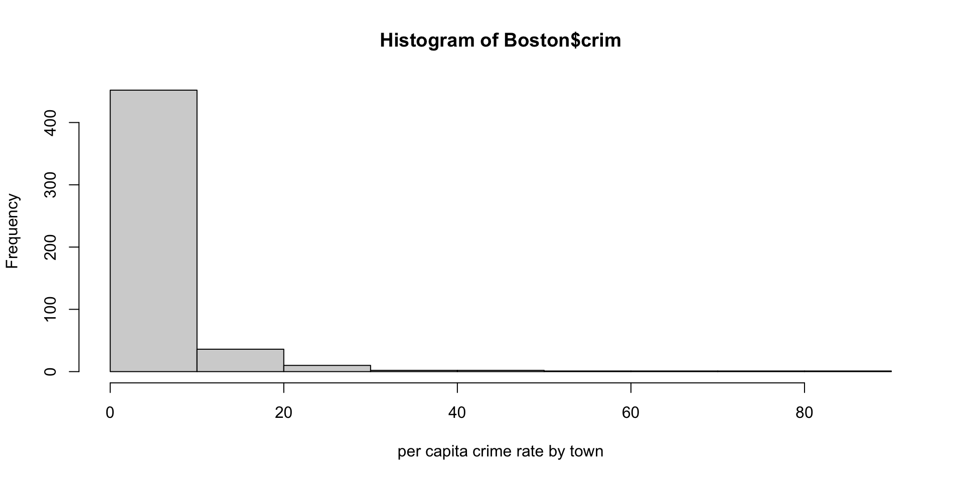
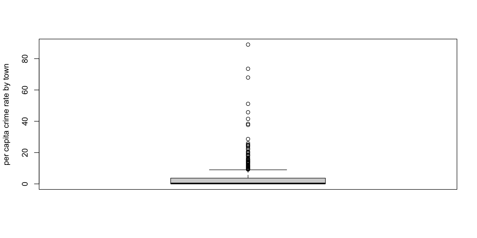
crim	per capita crime rate by town
zn	proportion of residential land zoned for lots over 25,000 sq.ft.
indus	proportion of non-retail business acres per town
chas	Charles River dummy variable (= 1 if tract bounds river; 0 otherwise)
nox	nitric oxides concentration (parts per 10 million)
rm	average number of rooms per dwelling
age	proportion of owner-occupied units built prior to 1940
dis	weighted distances to five Boston employment centres
rad	index of accessibility to radial highways
tax	full-value property-tax rate per $10,000
ptratio	pupil-teacher ratio by town
lstat	% lower status of the population
medv	Median value of owner-occupied homes in $1000’s

Per capita crime rate by town

Histogram

hist(Boston$crim, xlab = vardesc[1])

Per capita crime rate by town

Boxplot

boxplot(Boston$crim, ylab = vardesc[1])

Per capita crime rate by town

This variable has a strongly right skewed distribution
Mean and median will have very different interpretations in this situation

mean(Boston$crim)

[1] 3.613524

median(Boston$crim)

[1] 0.25651

Robust or outlier-resistant statistics

Measure	Type	Sensitive to Outliers?	Notes
Mean	Center	Yes	Strongly affected by extreme values
Median	Center	No	Robust; not affected by outliers
Mode	Center	No	Not affected by outliers
Range	Spread	Yes	Determined by min and max values
Variance	Spread	Yes	Squared deviations amplify outliers
Standard Deviation	Spread	Yes	Derived from variance; sensitive
Interquartile Range	Spread	No	Only uses middle 50% of data

Summary

Describing distributions

Descriptive statistics help us understand the center, spread, and shape of data
Use mean, median, and mode for measures of center; range, standard deviation, and IQR for spread
Frequency and proportion tables summarize categorical variables
Visualizations (histograms, boxplots, barplots) reveal distribution and outliers
Always consider the impact of outliers and choose robust statistics when appropriate

Week 3: Descriptive Statistics and Summarizing Data

Refresher I

Class and type

Refresher II

Basic structure

Refresher III

Subsetting a column from a data frame

Refresher IV

Type coercion

Refresher V

Aside about memory efficiency

What does the dataset look like?

What are some questions we might pose about these data?

Interlude: statistical terminology refresher

What is a population?

What is a distribution?

What is a sample?

What is a statistic?

Descriptive statistics

What are Descriptive Statistics?

Types of Descriptive Statistics

Summarizing Numeric Data

Measures of Center

Measures of Spread

Summarizing Categorical Data

Frequency Tables

Back to the Diamonds Dataset

Recalling the structure

Diamond price

Measures of center

Diamond price

Measures of spread

Diamond price

Measures of spread

Diamond price

Shape

Diamond price

Shape

Diamond cut quality

The cut variable

Diamond cut quality

Frequency table

Diamond cut quality

Proportion table (relative frequency)

Outliers and outlier-resistant summaries

Boston housing data

Per capita crime rate by town

Histogram

Per capita crime rate by town

Boxplot

Per capita crime rate by town

Robust or outlier-resistant statistics

Summary

Describing distributions

The `cut` variable