Week 13: Logistic Regression & AI-assisted Workflows

Part 1: Logistic regression

Overview

  • Recall from Week 9: in linear regression, we modeled a continuous response \(Y\) as \[Y = \beta_0 + \beta_1 X + \epsilon, \] where \(\epsilon\) was a normally distributed error term. Estimation and inference used least squares and normal-error assumptions.

New question

What if the response \(Y\) is binary (0/1)?

  • The “mean” of \(Y\) is now a probability that \(Y = 1\)
  • Residuals cannot possibly be normal in this situation
  • Predictions for the mean could fall outside \((0, 1)\)

Better model: logistic regression…

Motivating example: Dose–toxicity modeling

We consider an early-phase Oncology clinical trial where cohorts of patients receive increasing drug doses. The binary outcome \(Y\) indicates whether a dose-limiting toxicity (DLT) occurred (1 = yes, 0 = no).

Construct dose-toxicity dataset (dlt_data) and display empirical rates.
dlt_data <- tibble::tibble(
  dose = c(1, 2.5, 5, 10, 20, 25),
  num_patients = c(3, 4, 5, 4, 6, 2),
  num_toxicities = c(0, 1, 0, 1, 1, 2)
) |>
  dplyr::mutate(empirical_rate = num_toxicities / num_patients)

dlt_data |>
  gt() |>
  tab_header(title = "Drug A Dose–Toxicity Data (DLTs)") |>
  cols_label(
    dose = "Dose A (mg)",
    num_patients = "Patients",
    num_toxicities = "DLTs",
    empirical_rate = "Proportion of DLTs"
  ) |>
  fmt_percent(columns = empirical_rate, decimals = 1) |>
  fmt_number(columns = c(num_patients, num_toxicities), decimals = 0) |>
  tab_style(
    style = cell_fill(color = "#f2f7ff"),
    locations = cells_column_labels()
  ) |>
  opt_table_font(font = "Arial")
Drug A Dose–Toxicity Data (DLTs)
Dose A (mg) Patients DLTs Proportion of DLTs
1.0 3 0 0.0%
2.5 4 1 25.0%
5.0 5 0 0.0%
10.0 4 1 25.0%
20.0 6 1 16.7%
25.0 2 2 100.0%

Fitting logistic regression in R

fit_dose <- glm(cbind(num_toxicities, num_patients - num_toxicities) ~ I(log(dose)),
                data = dlt_data,
                family = binomial())
summary(fit_dose)

Call:
glm(formula = cbind(num_toxicities, num_patients - num_toxicities) ~ 
    I(log(dose)), family = binomial(), data = dlt_data)

Coefficients:
             Estimate Std. Error z value Pr(>|z|)  
(Intercept)   -3.3528     1.6537  -2.027   0.0426 *
I(log(dose))   0.9309     0.6495   1.433   0.1518  
---
Signif. codes:  0 '***' 0.001 '**' 0.01 '*' 0.05 '.' 0.1 ' ' 1

(Dispersion parameter for binomial family taken to be 1)

    Null deviance: 10.159  on 5  degrees of freedom
Residual deviance:  7.476  on 4  degrees of freedom
AIC: 16.751

Number of Fisher Scoring iterations: 5

Making predictions

# Predict the probability of a DLT for dose = 25
predict(fit_dose, newdata = data.frame(dose = c(1, 2.5, 5, 10, 20, 25)), type = "response")
         1          2          3          4          5          6 
0.03380373 0.07586928 0.13533291 0.22981219 0.36259074 0.41182696 

Plotting the predictions

Plot on probability scale
# Probability scale
dose_grid <- tibble::tibble(dose = seq(min(dlt_data$dose), max(dlt_data$dose), length.out = 100)) |>
  dplyr::mutate(p_hat = predict(fit_dose, newdata = dplyr::cur_data(), type = "response"))

ggplot(dlt_data, aes(x = dose, y = empirical_rate)) +
  geom_point(size = 3, color = "#1f77b4") +
  geom_line(data = dose_grid, aes(y = p_hat), color = "#d62728", linewidth = 1) +
  scale_y_continuous(labels = scales::percent_format(accuracy = 1)) +
  scale_x_log10() + 
  labs(title = "Probability scale",
       x = "Dose A (mg)",
       y = "Probability of DLT") +
  theme_minimal()

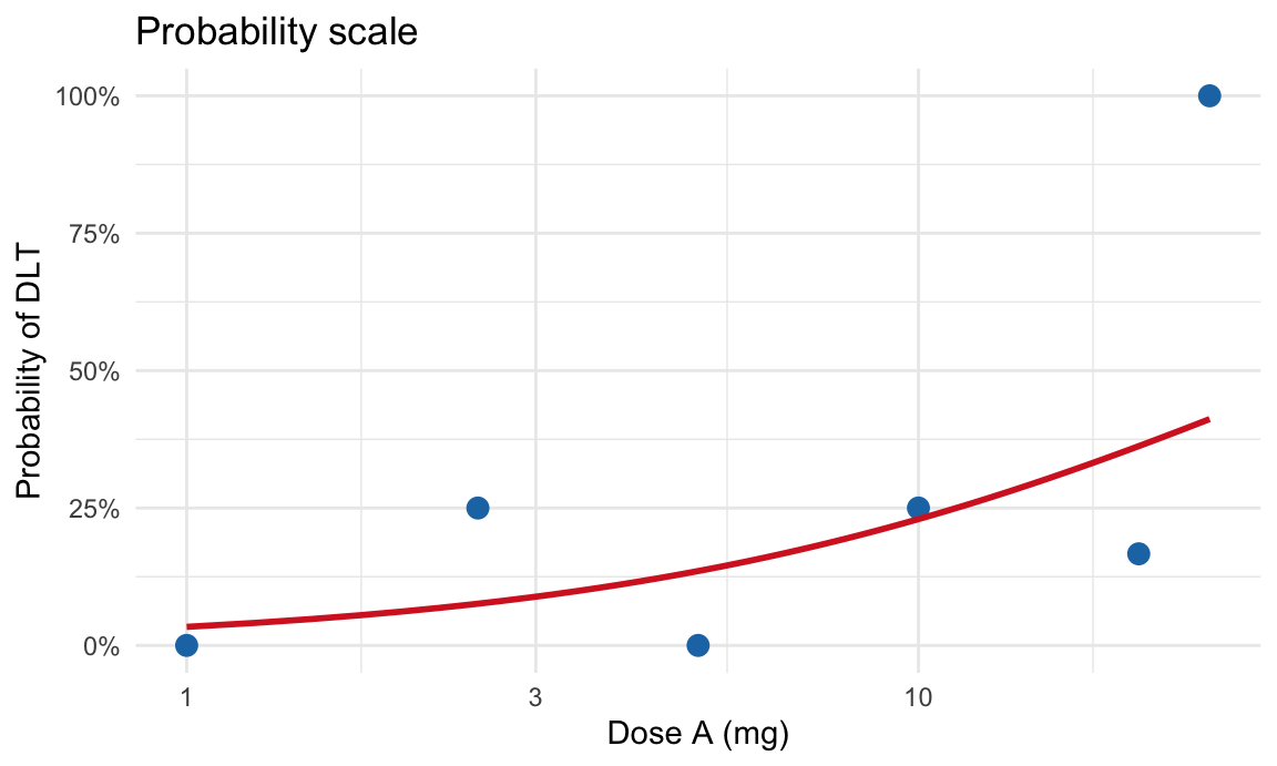
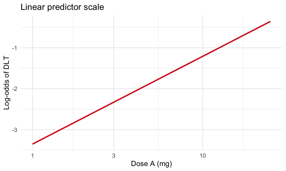
Plot on linear predictor scale
# Linear predictor (log-odds) scale
dose_grid_lp <- tibble::tibble(dose = seq(min(dlt_data$dose), max(dlt_data$dose), length.out = 100))
pred_lp <- predict(fit_dose, newdata = dose_grid_lp, type = "link", se.fit = TRUE)
dose_grid_lp$eta_hat <- as.numeric(pred_lp$fit)

ggplot(dose_grid_lp, aes(x = dose, y = eta_hat)) +
  geom_line(color = "#d62728", linewidth = 1) +
  scale_x_log10() + 
  labs(title = "Linear predictor scale",
       x = "Dose A (mg)",
       y = "Log-odds of DLT") +
  theme_minimal()

Generalized linear models (GLMs)

  • A unified framework that includes linear, logistic, and Poisson regression (among others).
Model Typical data R syntax Link function
Linear regression Continuous outcomes (approximately normal residuals) lm(y ~ x, data = df)
glm(y ~ x, data = df, family = gaussian())
identity
Logistic regression Binary 0/1 outcomes or successes/trials glm(y ~ x, family = binomial(), data = df)
glm(cbind(successes, trials - successes) ~ x, family = binomial(), data = df)
logit
Poisson regression Count data glm(y ~ x, family = poisson(), data = df) log

Part 2: AI-assisted workflows with R

Where do humans1 need AI?

  • Learning with AI
  • Code generation
  • Documentation and testing of code

Where does AI need humans?

  • Trust
  • Integration
  • Taste

Trust

  • How do your stakeholders know a statistical result is trustworthy?
  • Who is accountable for correctness? Must be a human
  • Must be able to identify issues in e.g. statistical ideas and/or generated code

Integration

  • Effective/impactful use of AI requires a new class of experts, e.g.
    • Technical experts: technology underlying LLMs is itself statistical (models trained on massive data, predicting the next word)
    • Facilitators: people who understand what tools are available and can connect them to solve practical problems

Taste

  • Knowing what to ask (prompt engineering)
  • Discriminating between good/useful output, and poor/unsuitable output
  • Knowing when AI should not be used

What does it mean for me and you?

  • Need knowledge and experience to develop taste, e.g.
    • Statistical knowledge
    • R programming experience
  • Need to learn how and when to effectively work with AI