Week 1: Introduction

Getting started

Acquaintances

  • About me
  • About you
  • About the course

Course goals

  • Attain basic programming fluency in R
  • Use R to:
    • Manipulate and summarize data
    • Apply statistical techniques to learn from data
  • Strengthen your skills at:
    • Making data-based insights to real-world problems
    • Communicating findings clearly
    • Assessing strength of statistical arguments

About R

  • Prehistory: the S language
    • S was developed by John M. Chambers at Bell labs in the 1980s
    • Focus was on data analysis and graphics
    • S version 3 was released alongside the influential book Statistical Models in S (1992) by Chambers and Trevor Hastie (a highly influential statistician in the area of statistical and machine learning)
    • S was proprietary software distributed by Bell, later commercialized as S-PLUS
  • Development of R
    • R is a free open-source implementation of S
    • It was written by Ross Ihaka and Robert Gentlemen at the University of Auckland

Languages for modern data science

Contemporary landscape

  • Highly multi-lingual enviornment for practicing data scientists today: Python, R, Julia, etc.
  • Relative strengths of R
    • Popularity in the field of statistical reasearch (in some more applied sub-fields, like AI and Machine Learning, Python is ascendant)
    • Open-source extensions (“libraries”) include leading frameworks for data manipulation and visualization, and also for cutting edge new methodologies
  • Relative weaknesses of R
    • Speed and performance
    • Weak native object orientation

Glimpse of R in action

Example: R package download counts

Getting the data from cranlogs

  • We will work with data from various sources this semester
  • In this example, I will look at data related to download counts for a few R packages from CRAN (the most popular repository for open-source extensions in R)
  • I do not expect you to understand all this code
  • Goal is just to highlight the efficiency with which R can handle data-analysis tasks
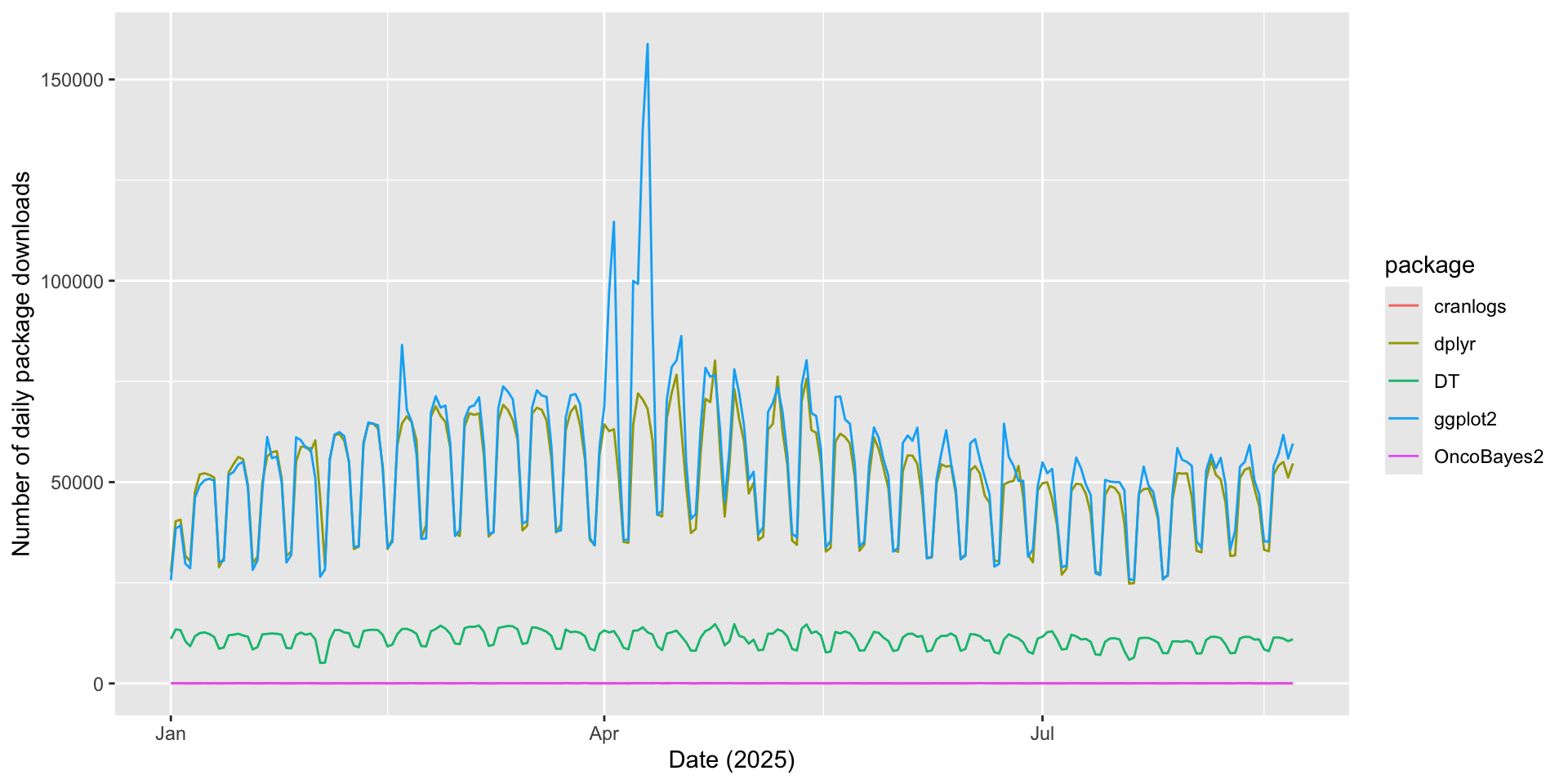
Getting some data about package download counts
library(cranlogs)

# list a few popular R packages
packages <- c("ggplot2", "dplyr", "cranlogs", "DT", "OncoBayes2")

# use the packageRank package function cranDownloads to 
# get some data about download counts in the past year
download_counts <- cranlogs::cran_downloads(
  packages = packages,
  from = "2025-01-01", to = "2025-08-22"
)

Example: R package download counts

Examine the data

Use the DT interface to DataTables.js for a paginated printout of the raw data
library(DT)
DT::datatable(download_counts, options = list(pageLength = 8))

Example: R package download counts

Visualize the data

  • R has extremely strong and user-friendly capabilities for graphics
  • Numerous popular packages, such as ggplot2, extend R’s usefulness in this area even further
Use ggplot2 to visualize the data on package-download counts
library(ggplot2)

ggplot(download_counts,
       aes(x = date, y = count, group = package, color = package)) +
  geom_path() +
  labs(x = "Date (2025)",
       y = "Number of daily package downloads")

Example: R package download counts

Manipulate and transform the data

  • R likewise has excellent facilities for storing and manipulating tabular data
Use dplyr to consolidate the daily counts into weekly counts
library(dplyr)

# sum counts for each package across each week of 2025
weekly_counts <- download_counts |>
  mutate(week = floor(difftime(date, "2024-12-31", units = "weeks")) +
            as.Date("2025-01-01")) |>
  group_by(package, week) |>
  summarize(count = sum(count), .groups = "drop")
Print the first several rows of the original data
knitr::kable(head(download_counts))
date count package
2025-01-01 11099 DT
2025-01-01 45 OncoBayes2
2025-01-01 34 cranlogs
2025-01-01 27657 dplyr
2025-01-01 25618 ggplot2
2025-01-02 13421 DT
Print the first several rows of the transformed data
knitr::kable(head(weekly_counts))
package week count
DT 2025-01-01 81713
OncoBayes2 2025-01-01 113
cranlogs 2025-01-01 258
dplyr 2025-01-01 270181
ggplot2 2025-01-01 256966
DT 2025-01-08 78110

Example: R package download counts

Visualize again with alternative time scales

Use ggplot2 to plot the download frequencies on both timescales
bind_rows(mutate(download_counts, time_unit = "daily", time = date),
          mutate(weekly_counts, time_unit = "weekly", time = week)) |>
  ggplot(aes(x = time, y = count, group = package, color = package)) +
  geom_path() +
  labs(x = "Date (2025)",
       y = "Number of package downloads per unit time") +
  facet_wrap(~ time_unit, labeller = "label_both", scales = "free")

Example: R package download counts

Leveraging more packages to simplify tasks

  • Some extensions to R are highly specialized for specific purposes (e.g. data-analysis tasks, types of data, types of models, etc.)
  • Many are community-supported, but some have more stable backing
  • Base R evolves slowly, while its extensions grow and adapt quickly
  • The right tool can make an otherwise difficult task very easy
Use specialized packages for time-indexed data, tsibble and lubridate, to manipulate ggplot2 download data over a longer timescale
library(tsibble)
library(lubridate)

ggplot_downloads <- cranlogs::cran_downloads(
  packages = "ggplot2",
  from = "2015-01-01", to = "2025-08-22"
) |>
  tsibble(index = "date") |>
  mutate(year = year(date),
         month = factor(month(date, label = TRUE, abbr = TRUE),
                        ordered = FALSE)) |>
  index_by(time = ~ yearmonth(.)) |>
  summarize(count = sum(count), month = first(month), year = first(year))

Example: R package download counts

Leveraging more packages to simplify tasks

Code for a basic plot is made extremely simple by using these specialist libraries
ggplot_plot <- fabletools::autoplot(ggplot_downloads, .vars = count)
ggplot_plot

Example: R package download counts

Fitting a linear regression model

  • R is designed for and heavily used by statisticians
  • It has strong native support for classical statistical techniques
# Simple linear regression of monthly download count on time (in months)
fit <- lm(count ~ time, data = ggplot_downloads)
summary(fit)

Call:
lm(formula = count ~ time, data = ggplot_downloads)

Residuals:
     Min       1Q   Median       3Q      Max 
-1510522  -302044   -73162   348538  1643740 

Coefficients:
              Estimate Std. Error t value Pr(>|t|)    
(Intercept) -1.108e+07  7.803e+05  -14.20   <2e-16 ***
time         6.738e+02  4.240e+01   15.89   <2e-16 ***
---
Signif. codes:  0 '***' 0.001 '**' 0.01 '*' 0.05 '.' 0.1 ' ' 1

Residual standard error: 539600 on 126 degrees of freedom
Multiple R-squared:  0.6671,    Adjusted R-squared:  0.6645 
F-statistic: 252.5 on 1 and 126 DF,  p-value: < 2.2e-16

Summary

  • R is awesome for people who love data
  • Base R was developed with statisticians in mind
  • Statistics has evolved very rapidly as a field in recent decades as computational power has advanced
  • Open-source extensions to R (“packages”) can dramatically simplify data-analysis tasks

Example: R package download counts

Visualizing the fit

Add the fitted line to the previous plot
# Simple linear regression of monthly download count on time (in months)
ggplot_plot + 
  geom_path(data = mutate(ggplot_downloads, pred = predict(fit)),
            aes(y = pred), color = "red")

Fireside chat

About the last example

  • Are you familiar with simple linear regression?
  • What (if anything) concerns you about the use of this technique in the last example?

Some more questions for you

Installing things

Software to install

  • R (free and open source)
  • RStudio IDE (free commercial software)
  • Quarto (free commercial software): “literate programming”

Step-by-step

  1. Go to https://cran.rstudio.com and download the latest version of R
  2. Go to RStudio Desktop download page and download RStudio Desktop
  3. Go to Quarto Getting Started and download Quarto

One more thing

  • For labs, we will use Quarto to render code and outputs into pdf documents.
  • This has one more prerequisite
    1. In RStudio, in the bottom-left pane, switch from the “Console” to the “Terminal” tab.
    2. Type in and run this command: quarto install tinytex

Lab 1

About labs

  • Labs will be in-class hands-on coding and/or data-analysis exercises
  • Most labs will entail editing and rendering a skeleton Quarto script I will provide to you
  • Instructions for the lab will be included in the script for the week

Lab 1

  • For Lab 1 you’ll start from this pdf: lab_1.pdf